Lab 5: Sorting, Velocity analysis and Stacking

Objective:

To sort the shot gathered data into CMP, picking appropriate stacking velocities and stacking all CMPs in order to reveal a true image of the subsurface.

Theory:

1. Common Midpoint Sorting:

Seismic data is acquired in the shot gather mode while most seismic data processing is performed in the CMP-offset mode so we need to sort the traces between these modes. For this purpose, we use stacking charts that is a chart in which the x-axis indicates the geophone location and the y-axis indicates the source location. It is used to sort the traces into various modes or gathers such as shot, receiver, offset, or CMP.

2.Velocity analysis

Different types of seismic velocities exist such as: the NMO, stacking, RMS, average, interval, and phase, group, and migration velocities. The velocities that can be derived reliably from the time-space (t−x) data are the NMO, RMS, and stacking velocities. In this practical we will use stacking velocities that will be used after NMO correction of the data. Our aim is to obtain velocities that flatten out hyperbolas (which mainly represent reflections) on CMP gathers.

To compute the stacking velocities we can use velocity spectrum and constant velocity stack.

Velocity spectrum is used to find the stacking velocity to each reflector by mapping the time-space data of a single CMP gather onto a velocity spectrum plane. The steps for this method are as below:

Selecting a CMP gather with relatively high SNR ratio. The CMP gather should be sorted in offset.
Determining the minimum (usually equals 0) and maximum (usually equals to the record length) t0 (vertical axis) that you want to analyse.
Determining the minimum, maximum, and increment of vs( horizontal axis) to be attempted.

Normal Moveout Correction

NMO correction corrects the additional travel time of from source to receiver for nonzero offset travel times by applying the stacking velocities to CMP traces. This is done to prepare the data for stacking and estimating the NMO velocity.

NMO is the time difference between TWT at an offset x≠zero and TWT at zero-offset.

ΔtNMO(x) = t(x) − t0

For single horizontal layer with constant velocity, t-x curve is hyperbola

𝑡2(𝑥)= 𝑡02+ 𝑥2 /𝑣2

The NMO correction can be shown as below:

𝑡𝑁(𝑥)=𝑡(𝑥)+ Δ𝑡𝑁𝑀𝑂(𝑥)≈𝑡0

tNMO(x) is subtracted from t(x) such that the two-way travel time at offset x, after NMO correction is approximately equal to t0

tNMO(x) = t(x) − tNMO(x) ≈ t0

If the correct NMO velocity is used for NMO correction, the event will be horizontally aligned at t = t0.
If a higher velocity is used for NMO correction, then the event will be under corrected (i.e., concave down).
If a lower velocity is used for NMO correction, then the event will be overcorrected (i.e., concave up).

3.Stacking:

Stacking objective is to eliminating coherent and incoherent noise in the data in order to enhance the SNR ratio and extract subsurface image approximation. The traces in the NMO-corrected CMP gather are summed up to produce one stacked trace that represents that CMP. The amplitude pf the stacked data can be sum or average of the traces.

Computer Assignment

1.Display using the wiggle variable area mean the 18 shot gathers and the 65 CMP gathers, one at a time and analyze this carefully with Figure 5.3. You can use the MATLAB capabilities to make a movie for each.

2.Select CMP gather number 250 along with its stacking time and velocities and then:

• Add 1500 ft/s to the velocity values and perform NMO correction.

• Subtract 1500 ft/s to the velocity values and perform NMO correction.

3.What can you realize from both NMO corrected CMP gathers?

load SeismicData_gain_bpf_sdecon_gain.mat
[Dsort ,Hsort] = ssort(Ds_gain ,H);
save SeismicData_gain_bpf_sdecon_gain_sorted.mat Dsort Hsort

[cmps ,fold_cmp ]= extracting_cmp_fold_num(Dsort ,Hsort);
figure ,stem(cmps ,fold_cmp ,'k-')
xlabel('CMP numbers','FontSize' ,14)
ylabel('Fold','FontSize' ,14)
set(gca ,'YMinorGrid','on')

cmp_num =208;
[Dcmp, dt,t,cdp]= extracting_cmp(Dsort ,Hsort ,cmp_num); %error sebelum ni sebab position t salah, patut ada dt sebelum t tu.
scale =2;
figure ,mwigb(Dcmp ,scale ,cdp ,t)
xlabel (['CMP: ',num2str(cmp_num),''],'FontSize' ,14)
ylabel('Time(s)','FontSize' ,14)

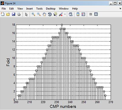
The fold (number of traces per CMP) versus the CMP numbers

From the result you can see that the data for CMP starts at 203 and it at CMP 235 it reaches the maximum fold of 18. The CMPs with low fold would affect the quality of velocity analyses and stacking. maximum number of samples can be obtained using full fold CMP gather 23.

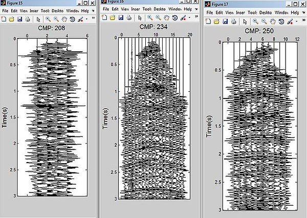
CMP Gathers

among three CMP gather, 208 has the lowest fold compared to 234 and 250. low fold gathers are unrealiable for interpretation,

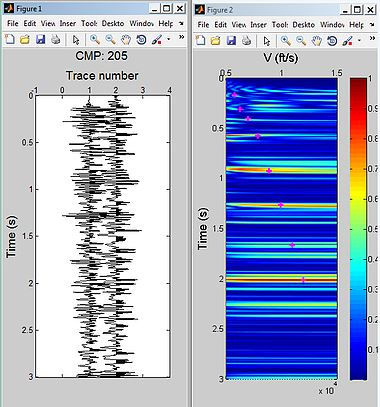
CMP gather 205 (left) and semblance plot (right)

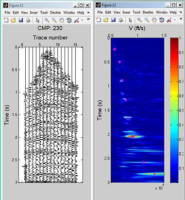
CMP gather 230 (left) and semblance plot (right)

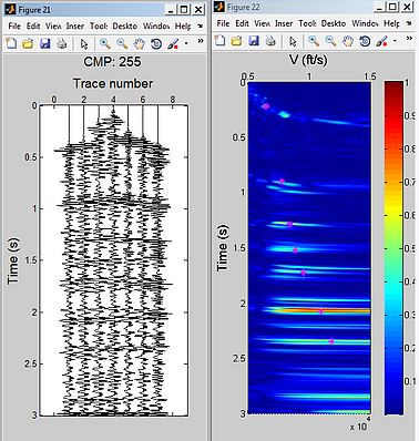
CMP gather 255 (left) and semblance plot (right)

low fold CMP gathers 205 shows the contours in the semblance plot are broad and flat taht means poor velocity discrimination.CMP 230, the contours is concentrated to a point in the semblance plot and velocity can be discriminated easier than 205.

CMP gathers and semblance plot : 205, 210, 215, 220, and 225.

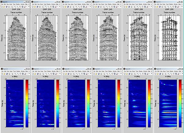
CMP gathers and semblance plot : 230, 235, 240, 245, 250, and 255.

forvelocity picking it is necessary to compare the semblance plot with the CMP gathers to ceck whether the picked velocity is optimum for flattening the gathers. picking velocity depends on size of the survey The more dense the interval, the more accurate the velocity analyses would be.