Seismic Data Processing
Lab 2: Seismic Data QC
Quality Control of Seismic Data
When seismic data is acquired and recorded, various quality control (QC) steps (called preprocessing in signal processing) are necessary to carry the remaining seismic data processing forward and ultimately obtain an accurate seismic image of subsurface structures. The QC process involves a series of steps to condition the data and prepare it for further quality control and processing. they can be listed as below:
-
De-multiplexing: The data is transposed from the recording mode, where each record contains the same time sample from all receivers, to the trace mode where each record contains all time samples from one receiver. This is usually done in the field.
-
Reformatting: The data is converted from one seismic digital format (e.g., SEG-Y) to another format that is convenient to the processing software and used throughout the processing flow (e.g., MATLAB).
-
Setup of field geometry: The geometry of the field is written into the data (trace headers) in order to associate each trace with its respective shot, offset, channel, and CMP.
-
Trace editing: During this step, bad traces, or parts of traces, are muted (zeroed) or killed (deleted) from the data and polarity problems are fixed.
-
Gain application: Amplitude corrections are applied to account for amplitude losses due to spherical divergence and absorption.
-
Application of field statics: In land surveys, elevation statics are applied to bring the sources and receivers to a common datum level. This step can be delayed until the static correction process where better near-surface velocities might be available.
Trace Editting
Objective :
To edit or remove noisy traces
Theory :
noise in seismic data is one of the problems we often face.; the noisy traces should be removed stacking to generate a good quality image. These traces can be the result of dead geophones, cultural noise and poor near-surface conditions.
Practical :
%% Load Seismic Data
clear,clc,close all
load SeismicData
% Choose shot number
shot_num =16;
% Extract the shot gather from the data matrix,D and header information
% from the structure matrix,H
p=0;
[Dshot ,dt ,dx ,t,offset ] = extracting_shots(D,H,shot_num ,p);
%% Display your shot gather as a wiggle as input
scale =1;
mwigb (Dshot ,scale ,offset ,t)
xlabel ('Offset (ft)','FontSize' ,14)
ylabel ('Time(s)','FontSize' ,14)
title('Before Muting','FontSize' ,14)
%% Muting
[i,j]= find(D==max(max(D)));
D(:,j)=0;
%% Display your shot gather as a wiggle as output
p=0;
[Dshot ,dt ,dx ,t,offset ] = extracting_shots(D,H,shot_num ,p);
scale =1;
figure
mwigb (Dshot ,scale ,offset ,t)
xlabel ('Offset (ft)','FontSize' ,14)
ylabel ('Time(s)','FontSize' ,14)
title('After Muting,'FontSize' ,14)
Before muting, in shot record 16, from 2.25 to 3 ms, trace 31 has an unusual, irregular trace. After muting, by muting the trace and interpolating it after, we managed to remove the bad trace entirely and replace it with a nomal trace.
a trace with abnormal amplitude exist in shot record 16 and it has been noticed that the bad trace is in trace 31. we zero the trace and interpolate the trace by averaging the properties from the neighbouring traces to remove anomoly and we replace the removed trace by normlized trace.
Correction for amplitude losses
Objective :
To compensate for amplitude losses due to transmission loss, geometric divergence and absorption.
Theory :
-
Transmission loss: This occurs at each geological reflector where part of the propagating seismic incident waves will be reflected, refracted, diffracted, scattered, etc. There is no loss here in terms of the mechanical energy since the lost energy merely travels somewhere else.
-
Geometric divergence: As the seismic wave spreads out from its source, its amplitude decays by an amount proportional to the reciprocal of the distance from the source to the location of the propagating seismic wave.
-
Absorption: This occurs where the seismic energy is converted into heat by friction. This loss is proportional to the exponential of the distance from the source.
amplitude correction or gain must be applied to seismic data sets at various stages. At the preprocessing stage, you may want to correct amplitudes due to geometric divergence as well as absorption losses. Also, whenever you want to display seismic data, you may want to boost weak signals by adding more gain to the data. There exist data independent and dependent amplitude correction schemes. The data-independent scheme corrects the amplitudes using a common scaling function to all the traces such as the gain through multiplication by a power of time using:
where f (t) is the seismic trace amplitude to be corrected, t is the time independent variable, and α is the power of time which controls the change in the amplitude of f(t). Another commonly used function is the exponential gain function correction:
Practical :
to have better visualisation of our data with a more normalized amplitude ]we correct amplitude losses in the early stages of processing .
%% Load Seismic Data
clear,clc,close all
load SeismicData
% Choose shot number
shot_num =8;
% Extract the shot gather from the data matrix,D and header information
% from the structure matrix,H
p=0;
[Dshot ,dt ,dx ,t,offset ] = extracting_shots(D,H,shot_num ,p);
%% Display your shot gather as a wiggle as input
scale =1;
mwigb (Dshot ,scale ,offset ,t)
xlabel ('Offset (ft)','FontSize' ,14)
ylabel ('Time(s)','FontSize' ,14)
title('Before Gain','FontSize' ,14)
%% Amplitude Gain
pow =2; %power value
T=0; %time correction
Dg=iac(Dshot ,t,pow ,T);
%% Display your shot gather as a wiggle as output
scale =1;
figure
mwigb (Dg ,scale ,offset ,t)
xlabel ('Offset (ft)','FontSize' ,14)
ylabel ('Time(s)','FontSize' ,14)
title('After Gain','FontSize' ,14)
tnum =33;
%seis_env_dB(Dshot ,Dg ,t,tnum)
%seis_env_dB(Dshot ,Dg ,t)
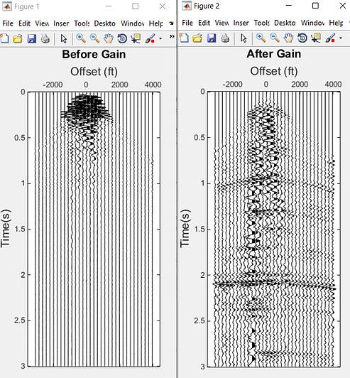
in shot record 33, the amplitude is concentrated in the shallower section only. The loss in amplitude towards the deeper section can be due to geometrical spreading,. After gain, the amplitude is balanced throughout the record length.
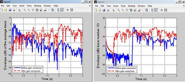
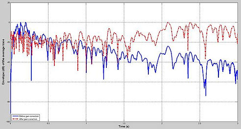
blue line shows before gain, the average amplitude envelope the traces shows the \ decrease in amplitude over time.After gain (red line), we can observe the amplitude is more balanced .gain in deeper section can be observed .
clc,clear,close all
load SeismicData.mat
shot_num =8;
p=0;
[Dshot ,dt ,dx ,t,offset ]= extracting_shots(D,H,shot_num ,p);
%% AGC Gain with RMS
agc_gate =0.5;
T=2; %normalize with rms value
Dg=AGCgain(Dshot ,dt ,agc_gate ,T);
scale =1;
figure, mwigb (Dg ,scale ,offset ,t)
xlabel ('Offset (ft)','FontSize' ,14)
ylabel ('Time(s)','FontSize' ,14)
title ('Normalize using RMS value','FontSize',14)
%% Display amplitude envelope gain in dB
tnum =33;
seis_env_dB(Dshot ,Dg ,t,tnum)
seis_env_dB(Dshot ,Dg ,t)
clc,clear,close all
load SeismicData.mat
shot_num =8;
p=0;
[Dshot ,dt ,dx ,t,offset ]= extracting_shots(D,H,shot_num ,p);
%% AGC Gain with trace amplitude
agc_gate =0.5;
T=1; %normalize with trace amplitude
Dg=AGCgain(Dshot ,dt ,agc_gate ,T);
scale =1;
figure, mwigb (Dg ,scale ,offset ,t)
xlabel ('Offset (ft)','FontSize' ,14)
ylabel ('Time(s)','FontSize' ,14)
title ('Normalize using trace amplitude','FontSize',14)
%% Display amplitude envelope gain in dB
tnum =33;
seis_env_dB(Dshot ,Dg ,t,tnum)
seis_env_dB(Dshot ,Dg ,t)
%% AGC Gain with RMS
agc_gate =0.5;
T=2; %normalize with rms value
Dg=AGCgain(Dshot ,dt ,agc_gate ,T);
scale =1;
figure, mwigb (Dg ,scale ,offset ,t)
xlabel ('Offset (ft)','FontSize' ,14)
ylabel ('Time(s)','FontSize' ,14)
title ('Normalize using RMS value','FontSize',14)
%% Display amplitude envelope gain in dB
tnum =33;
seis_env_dB(Dshot ,Dg ,t,tnum)
seis_env_dB(Dshot ,Dg ,t)
Computer Assignment
1. With α, β = 1.8, 2.2 and 3.4, use both the multiplication by a power of time and the exponential gain function corrections on the selected shot gathers. Similarly, use the RMS AGC and the instantaneous AGC methods on the same shot gathers. Display and compare your results with the data before applying the required amplitude corrections. In your opinion, which method results in the best amplitude correction? Why?
clear all; close all;
%% Trace editing (muting) %%
load SeismicData.mat;
shot_num =16;
p=0;
[Dshot16 ,dt ,dx ,t,offset ] = extracting_shots(D,H,shot_num ,p);
scale =1;
figure ,mwigb (Dshot16 ,scale ,offset ,t);
xlabel ('Offset (ft)','FontSize' ,14);
ylabel ('Time(s)','FontSize' ,14);
[i,j]= find(D==max(max(D)));
D(:,j)=0;
[Dshot16mute ,dt ,dx ,t,offset ] = extracting_shots(D,H,shot_num ,p);
scale =1;
figure ,mwigb (Dshot16mute ,scale ,offset ,t);
xlabel ('Offset (ft)','FontSize' ,14);
ylabel ('Time(s)','FontSize' ,14);
%% Correction to amplitude losses %%
load SeismicData.mat;
shot_num =8;
p=0;
[Dshot8 ,dt ,dx ,t,offset ]= extracting_shots(D,H,shot_num ,p);
pow =2; %power value
T=0; %time correction
Dg8=iac(Dshot8 ,t,pow ,T);
%before gain
figure ,mwigb (Dshot8 ,scale ,offset ,t);
xlabel ('Offset (ft)','FontSize' ,14);
ylabel ('Time(s)','FontSize' ,14);
%after gain
figure ,mwigb (Dg8 ,scale ,offset ,t);
xlabel ('Offset (ft)','FontSize' ,14);
ylabel ('Time(s)','FontSize' ,14);
tnum =33;
seis_env_dB(Dshot8 ,Dg8 ,t,tnum) %trace 33
seis_env_dB(Dshot8 ,Dg8 ,t) %average trace
agc_gate =0.5;
T=1; %normalize with trace amplitude
Dg8traceamp=AGCgain(Dshot8 ,dt ,agc_gate ,T);
figure ,mwigb (Dg8traceamp ,scale ,offset ,t);
xlabel ('Offset (ft)','FontSize' ,14);
ylabel ('Time(s)','FontSize' ,14);
seis_env_dB(Dshot8 ,Dg8traceamp ,t,tnum) %tracenum
seis_env_dB(Dshot8 ,Dg8traceamp ,t) %average trace
agc_gate =0.5;
T=2; %normalize with trace rms value
Dg8RMS=AGCgain(Dshot8 ,dt ,agc_gate ,T);
figure ,mwigb (Dg8RMS ,scale ,offset ,t);
xlabel ('Offset (ft)','FontSize' ,14);
ylabel ('Time(s)','FontSize' ,14);
seis_env_dB(Dshot8 ,Dg8RMS ,t,tnum) %tracenum
seis_env_dB(Dshot8 ,Dg8RMS ,t) %average trace
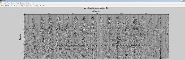
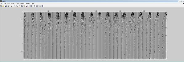
Shot record 11 to 14 before RMS AGC
Shot record 11 to 14 after RMS AGC
the shot gathers before RMS AGC shows concentration of amplitude at the beginning of the record length and decreases in deeper are. gathers after RMS AGCshows that the amplitude is equalized and reflections and noise are more clear.
RMS AGC i better because it considering the depth [G(t)] and \ how much correction should be applied.
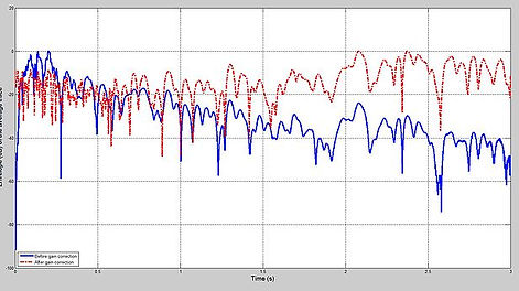
Envelope spectrum before and after RMS AGC for average of all traces (left) and for trace 33 (right).the amplitude decays as the time increases, but after applying gain correction, the amplitude is more balanced. When analyzed envelope spectrum of single trace 33, the inconsistent amplitude before is compensated by the gain correction.
3. Mute the bad traces of shot gather 16 as in Section 2 (Trace Editing). Then apply the method of multiplication by a power of time with α = 2.0 and all shot gathers and save the processed data with its header information as SeismicData_gain.mat to be used later on.
%% Load Seismic Data
clear,clc,close all
load SeismicData
% Choose shot number
shot_num =16;
% Extract the shot gather from the data matrix,D and header information
% from the structure matrix,H
p=0;
[Dshot ,dt ,dx ,t,offset ] = extracting_shots(D,H,shot_num ,p);
%% Display your shot gather as a wiggle as input
scale =1;
mwigb (Dshot ,scale ,offset ,t)
xlabel ('Offset (ft)','FontSize' ,14)
ylabel ('Time(s)','FontSize' ,14)
title('Before Muting','FontSize' ,14)
%% Muting
[i,j]= find(D==max(max(D)));
D(:,j)=0;
%% Display your shot gather as a wiggle as output
p=0;
[Dshot ,dt ,dx ,t,offset ] = extracting_shots(D,H,shot_num ,p);
scale =1;
figure
mwigb (Dshot ,scale ,offset ,t)
xlabel ('Offset (ft)','FontSize' ,14)
ylabel ('Time(s)','FontSize' ,14)
title('After Muting,'FontSize' ,14)
Shot record 16 before muting (left) and after muting (right).After muting, by muting the trace and interpolating it after, we managed to remove the bad trace entirely and replace it with a nomal trace.


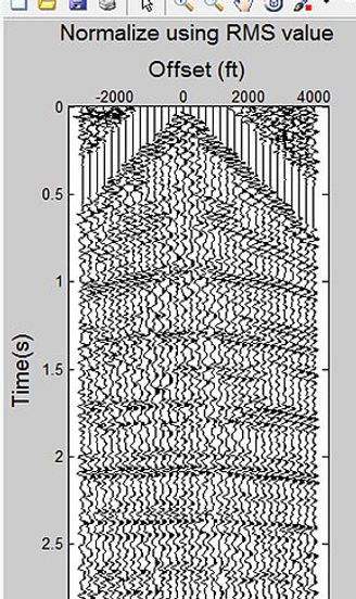
Normalization of amplitude using the RMS works by dividing the desired RMS scaler by the mean value of gate/window length and then multiplying it by theamplitudes of all the samples in the gate. The gain is dependant on the window used to compute the RMS scalar. RMS is sometimes discouraged because it takes into consideration the noise that exist in the selected window. By looking at the average amplitude envelope, the amplitude is proven to be balanced across the record length.
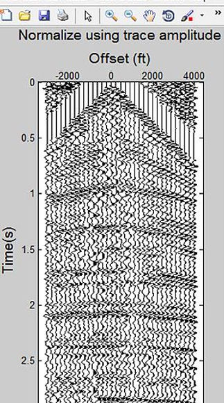
The instantaneous / trace amplitude works very similar to RMS value computation but by analyzing the amplitude of each signal. Trace amplitude computes the average amplitde for a series of signals, then applies the average amplitude onto each trace. The balance in amplitude is shown in the average amplitude envelope spectrum. The results are almost identifical with RMS value gain.