Lab 4: Seismic Deconvolution

Objective:

To increase the vertical resolution of the data by compressing the source wavelet.

Theory:

The deconvolution (inverse seismic convolutional model) Computes the earth’s reflectivity e(t) given the seismic trace s(t) and the source wavelet w(t). If the source wavelet is known, the deconvolution becomes deterministic. Whereas, if the source wavelet is not known, the deconvolution becomes statistical.

Spiking deconvolution compresses the source wavelet w(t) into a zero-phase spike of zero width. This leads to elimination the effect of the source wavelet and leaving only the effect of the Earth’s reflectivity in the seismogram.

Practical:

To perform spiking deconvolution in practice, some parameters need to be set. These parameters are listed as below:

• Auto-correlation window (w): This sets up the part of seismic trace from which we will select the elements of the autocorrelation matrix in the normal equations.

• Filter length (N): This sets up the length of the spiking filter h(n).

• Percent pre-whitening (ε): This sets up the amount of white random noise we want to include into our auto-correlation matrix to stabilize the solution of the normal equations.

Spiking Deconvolution of the data set:

We need to use M-functions spiking_decon.m and auto_correlation_map.m to perform spiking deconvolution filtering to calculate the auto-correlogram and for this purpose MATLAB m-file below is used.

Computer Assignment

Apply spiking deconvolution using the M-function spiking_decon.m followed by an instantaneous AGC to all the shot gathers and save the resultant data set (with its header) as SeismicData_gain_bpf_sdecon_gain.mat to be used in the coming chapters.
Use the formulation of Equation 4.13 to generalize the M-function spiking_decon.m so it can be used for predictive deconvolution process

clear all; close all;
load SeismicData_gain_bpf.mat;
shot_num =4:6;
p=1;
[Dshot ,dt ,dx ,t,offset ]= extracting_shots(Dbpf ,H,shot_num ,p);
[nt ,nx]= size(Dshot);
scale =5;
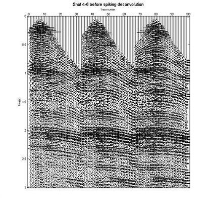
figure , mwigb(Dshot ,scale ,offset ,t)
xlabel('Trace number','FontSize' ,8)
ylabel('Time(s)','FontSize' ,8)
title('Shot 4-6 before spiking deconvolution','FontSize' ,14)
max_lag =0.2;
[Dauto ,lags ]= auto_correlation_map(Dshot ,max_lag ,dt);
scale =5;
figure , mwigb(Dauto ,scale ,offset ,lags)
xlabel('Trace number','FontSize' ,8)
ylabel('Time lag (s)','FontSize' ,8)
title('Auto-correlograms of shot gathers 4-6','FontSize' ,14)
mu=0.1;
Ds=spiking_decon(Dshot ,max_lag ,mu ,dt);
scale =5;
figure , mwigb(Ds ,scale ,offset ,t)
xlabel('Trace number','FontSize' ,8)
ylabel('Time (s)','FontSize' ,8)

title('Shot 4-6 after spiking deconvolution','FontSize' ,14)
Davg_before=mean(Dshot');
fs=1/dt;
[Davg_before ,f] = periodogram(Davg_before ,[] ,2*nt,fs);
Davg_before=Davg_before/max(Davg_before);
Davg_before =20* log10(abs(Davg_before));
Davg_after=mean(Ds');
[Davg_after ,f] = periodogram(Davg_after ,[] ,2*nt,fs);
Davg_after=Davg_after/max(Davg_after);
Davg_after =20* log10(abs(Davg_after));
fscale=linspace(-0.5 ,0.5 ,2* nt)/dt;
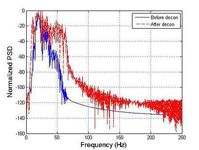
figure ,plot(f,Davg_before ,f,Davg_after ,'--r')
xlabel('Frequency (Hz)','FontSize' ,14)
ylabel('Normalized PSD','FontSize' ,14)
grid
legend('Before decon','After decon')
agc_gate =0.5;
T=1; %normalize with trace amplitude
Ds_gain=AGCgain(Ds ,dt ,agc_gate ,T);
scale =5;
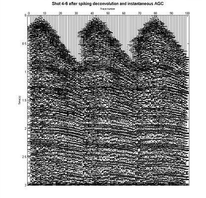
figure , mwigb(Ds_gain ,scale ,offset ,t)
xlabel('Trace number','FontSize' ,8)
ylabel('Time(s)','FontSize' ,8)
title('Shot 4-6 after spiking deconvolution and instantaneous AGC','FontSize' ,14)

Shot gather 4, 5 and 6 before applying spiking deconvolution

Shot gather 4, 5 and 6 after applying spiking deconvolution

after applying spiking deconvolution, the source wavelet becomes compressed and produces sharper wavelets.

we can notice that ringing effect also removed.

PSD of the average trace of shot gathers 4, 5 and 6 before and after spiking deconvolution.at higher frequencies increase in the signal power intensity is more obvious.

Shot gather 4, 5 and 6 after applying spiking deconvolution and instantaenous AGC